00
Executive summary
Summary of the project and main results
If support follows a net-decline ranking, the ranking is more closely related to store count than to closure risk. The category it ranks first overall in neighborhood commercial areas has a lower net-decline rate than comparable matched cells once cells are matched on size, though not at every size.
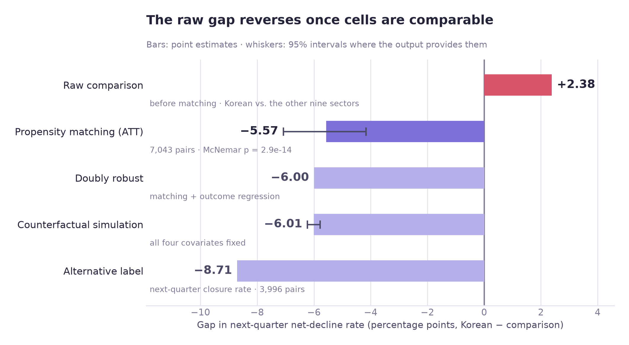
Raw comparison. Korean restaurants have the highest net-decline rate, 25.3% against 22.9% for the other nine food categories, pooled over 12 quarters in neighborhood commercial areas (first in only 3 of the 12 quarters taken individually). If support is allocated by a ranking like this, a gap like that could influence who receives support such as consulting or emergency loans. This is a hypothetical use case: net decline is this project's own label, and the page does not assume that any agency allocates support this way.
Tests of the raw gap
| Test | Result | What it means |
|---|---|---|
| Permutation test · 1,000 shuffles | p = 0.344 | The top category's lead over the all-ten average is +1.70 pp; picking the maximum of ten categories alone produces +1.49 pp on average, so 88% of that lead is what selecting the maximum alone would produce |
| Propensity matching · 7,043 pairs | −5.57 pp | Among matched, comparable cells, the sign of the difference reverses |
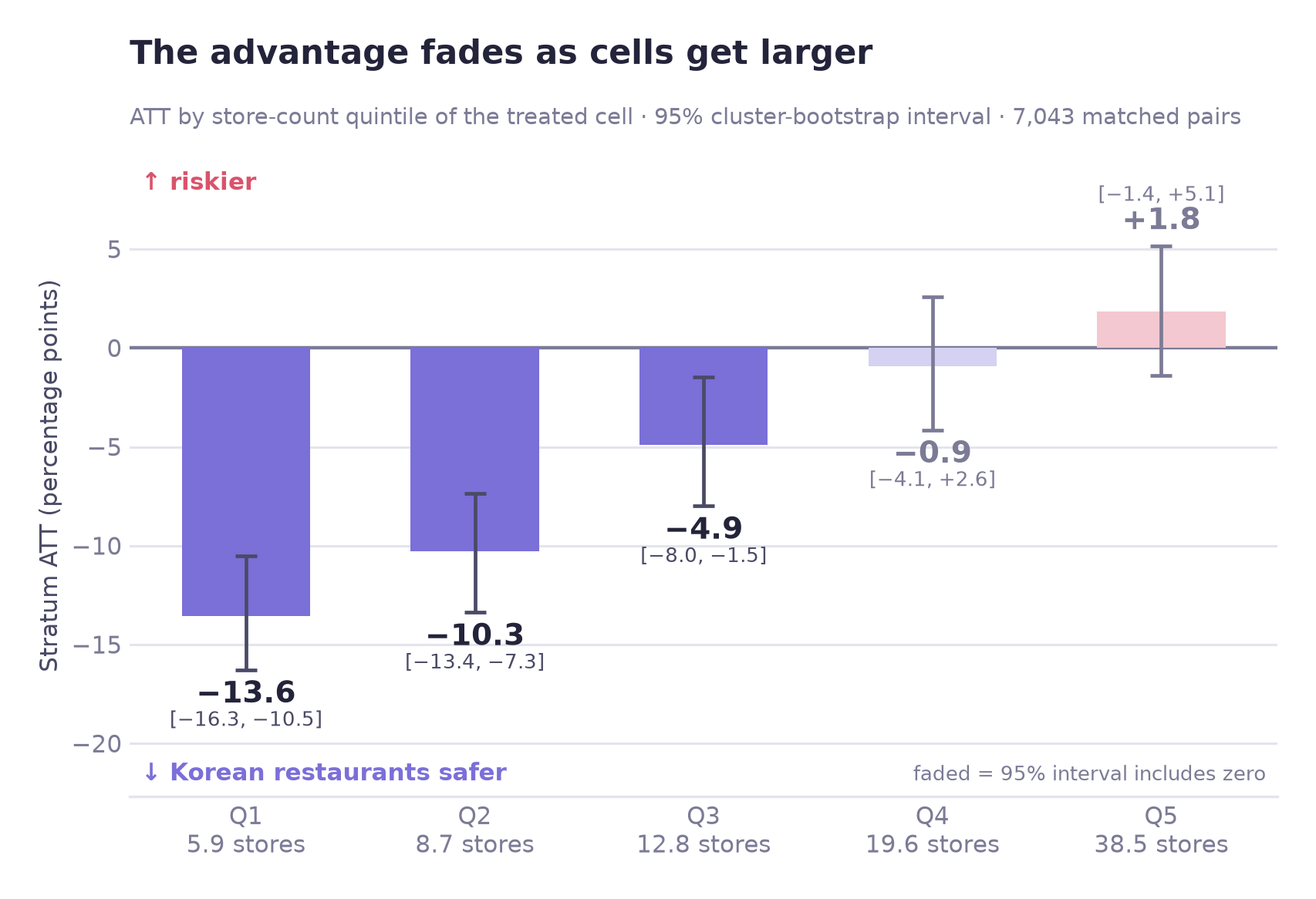
| Woolf homogeneity test | p < .0001 | The matched average combines estimates that differ across size bands: clearly negative in the three smallest bands, with intervals that include zero in the two largest |
Key findings
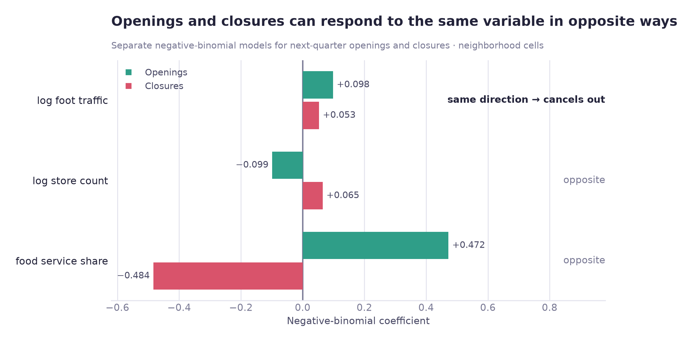
Store count alone accounts for almost all of the modeled reversal (−5.84 pp vs −6.01 pp with all four covariates held fixed). Foot traffic shows no significant association with net decline once store count and the other covariates are held fixed (AME +0.72 pp, p = 0.078; without store count it is strongly significant: AME +3.97 pp with foot traffic alone, +2.66 pp with area size and attracting facilities added, both p < 0.0001). It is associated with more openings and more closures, so the two largely cancel in the subtraction. The data do not show a busy district to be a safe one; the pattern is consistent with faster turnover.
The label decomposes exactly. Net decline = an event occurred × that event netting negative. Store count is strongly associated with the first term and has a small, non-significant coefficient in the second, so the label mainly reflects how often an opening or closure occurs rather than the direction of the balance once one occurs.
Seoul's change-indicator HL group (label in the source file: "contracting") has lift 0.937 for next-quarter net decline in the single validation quarter tested. The indicator grades each commercial area HH/HL/LH/LL by comparing the average operating months of its surviving and its closed businesses with Seoul-wide averages; HL means survivors' average is above Seoul's and closed businesses' is below. A lift below 1 means HL cells had a slightly lower net-decline rate than the average cell (24.3% against 26.0%). This tests one grade against this project's own label, which is not the indicator's published purpose, so it does not speak to the indicator's other uses.
The model's advantage appears at the operating point rather than in overall metrics. Top-50 precision is 0.780 against 0.380 for a store-count rule in the validation quarter, and the two lists overlap by only 4%, so 48 of the 50 flagged cells are ones the store-count rule does not list.
One result is not reported as performance evidence: the closure-count model's 0.915 category rank correlation, which rests on 10 categories in one validation quarter. Single-quarter rankings of the net-decline label were also noisy (see the checks in the methodology section).
Recommendation
Cell-level scores instead of category ranks
Net decline should not be used as a standalone measure of vulnerability. Closures per store can be shown beside it. If support were allocated by risk, a score at the level of one neighborhood commercial district × one food category is better supported by this analysis than an industry-level rank.
At a glance
01
Overview
Scope of the analysis and why it matters
Seoul's Commercial District Analysis Service publishes store openings and closures for every commercial district × food category in its quarterly tables, and a separate change indicator (HH/HL/LH/LL, a grade per commercial district based on the operating months of surviving and closed businesses relative to Seoul-wide averages; see section 06). It does not publish a net-decline flag. This project defines a cell's next-quarter net decline as closures outnumbering openings. The use case below is an assumption: if a district officer ranked food categories by that flag when deciding where consulting and emergency loans go, the ranking would have the properties tested below. The page does not claim that any agency allocates support this way.
This project examines whether such a ranking reflects closure risk or mainly store count, using 13 quarters of Seoul commercial-district data (12 labeled), 67,475 cells across all four area types, ten food categories, with propensity matching, regression and forecasting methods.
This is a team project. This page covers my work on hypothesis H2, the second supporting question and the connected forecasting and operational evaluation; the project's main question and H1 were handled by other teammates and are outside this page.
The unit of analysis
A cell is one commercial district × one food category × one quarter. Everything on this page is measured at that unit unless stated otherwise.
Two similar words
Commercial district is one trade area in the commercial-district boundary table (1,650 of them). City district is one of Seoul's 25 boroughs. They are not interchangeable, and the difference matters for the recommendation.
Why it matters. If the gap comes from size confounding, a category-level allocation would be better replaced by cell-level allocation conditioned on size. If it does not, a category-level ranking would remain reasonable.
02
Business question
Assumed use case and research questions
Korean restaurants rank #1 on the pooled net-decline rate in neighborhood commercial areas (first in 3 of the 12 quarters taken one by one); the ranking is computed in this project from Seoul's opening and closure counts. They are also the largest category in neighborhood districts, averaging 21.3 stores per cell against 10.3 for the other nine. Larger cells have more opening and closure events, and more events give more opportunities for closures to exceed openings.
Main question
Does controlling for commercial scale and foot traffic change the apparent difference in net-decline risk between Korean restaurants and other food categories?
Stated as a hypothesis before the analysis: matching on those two variables will narrow the gap.
Sub-question
Among sales, foot traffic and store density, which commercial characteristics are associated with next-quarter net decline?
Foot traffic shows no significant association with net decline once store count and the other covariates are controlled (AME +0.72 pp, p = 0.078), though it is significant without that control.
Unit
cell
Cells (all four area types)
67,475
Labeled quarters
12
Positive rate
25.5%
03
Data
Sources, sample construction and data corrections
Source
Seoul Open Data Plaza · Commercial District Analysis Service tables (provider: Seoul Credit Guarantee Foundation; license: KOGL Type 1, attribution; copyright holder: Seoul Metropolitan Government), 2023 Q1 – 2026 Q1. Five datasets were merged into one panel, plus a sixth used only as an external benchmark:
| Dataset | What it contributes |
|---|---|
| Stores by Commercial District | Store counts, openings and closures, franchise split; the source of the label |
| Street-Level Population by Commercial District | Foot traffic by hour, weekday and age band |
| Commercial District Boundaries | Polygon area, coordinates, district type |
| Attraction Facilities by Commercial District | Attracting-facility count and subway-station count per commercial district |
| Estimated Sales by Commercial District | Estimated sales value and transaction counts |
| Commercial District Change Indicator | The city's own HH/HL/LH/LL grade per commercial district (average operating months of surviving and closed businesses compared with Seoul-wide averages). Used only as a baseline, in a single validation quarter, and never as a feature; testing it against net decline is not its published purpose |
The dataset was used for educational portfolio purposes. This page documents the part of the team project that I analysed (see the scope note in the overview).
From 995,377 rows to 67,475
| Stage | Rows | Why |
|---|---|---|
| Raw store table | 995,377 | All business categories |
| 10 food categories × 13 quarters | 160,352 | Scope |
| Label constructible | 147,138 | Needs a following quarter to label against |
| 5 or more stores per cell | 67,495 | See below |
| Analysis sample | 67,475 | Foot traffic and area valid; all four area types |
| Neighborhood commercial areas only | 34,647 | Raw gap, permutation, matching and stratified-ATT sample (7,043 matched pairs) |
A five-store floor −54.1% of rows
The main reason is the label rather than the sales data. As an arithmetic illustration, in a three-store cell one closure is a third of all stores, against about 3% in a 30-store cell. Such differences reflect small sample size rather than district decline, and keeping those rows would let a model learn to pick out small cells rather than risky ones.
Sales missingness points the same way: 45.4% overall, 7.1% at five stores or more, 100% at two or fewer. A rate of exactly 100% looks like a rule rather than attrition, but what that rule is could not be confirmed: no published suppression threshold was located. It is reported as an observation, not a cause.
The filter is on store count, a covariate, not on missingness. The label is observed for every cell either way, so this narrows the population rather than selecting on the outcome. The cost is 54.1% of rows, which is why every conclusion carries the scope note “cells with five or more stores.”
A column that changed meaning would have distorted category comparisons
In the 2023–24 files, store_count is not total stores; it is non-franchise stores. The 2025 schema renamed it and introduced a separate total. Two identities confirm it at a match rate of 1.0000.
Correcting the mapping moved the sample from 55,795 to 67,475 (+20.9%), and the increase differed greatly by category: chicken +390% against Korean +2%. Left uncorrected, franchise-heavy categories would have been undercounted, which matters directly for a comparison between categories.
Sales excluded from the matching covariates
Missingness differs by category, and category is the treatment variable. Including sales would drop control cells selectively, which could bias the match itself.
A three-layer guard on every join
A duplicated key does not raise an error; it silently multiplies rows. Key uniqueness was asserted before merging, the merge was run with a declared relation, and the row count was checked after.
04
Methodology
Analysis design and the checks applied to each result
The pipeline
| # | Step | Decision that mattered |
|---|---|---|
| 1 | Define the label | Net decline in quarter t+1, built inside each (district, category) group so no cell borrows another's future |
| 2 | Choose the test from the distribution | Normality failed in all 39 groups across three comparisons (commercial-area type 4/4, service category 10/10, city district 25/25), so Kruskal-Wallis was used rather than ANOVA |
| 3 | Test the gap against selection | Permutation test, because the treated category was selected as the maximum of ten |
| 4 | Make the groups comparable | 1:1 propensity matching inside a caliper, exact-matched on quarter, without replacement |
| 5 | Robustness checks on the result | Doubly robust estimation, counterfactual simulation, an alternative outcome label, and a split by size |
| 6 | Predict and benchmark | Rolling validation against a baseline ladder and against the city's own indicator |
Why matching rather than regression adjustment
Limited overlap is the main concern. The two groups differed by a full standard deviation in store count. A regression can report a coefficient by extrapolating into the region where no comparable control cell exists. Matching does not extrapolate: a treated cell with no partner is dropped and counted, so lack of overlap appears as a visible count rather than a silent extrapolation.
Regression was still used: it enters as the doubly robust estimator alongside the match, so both numbers are reported.
Why gradient boosting margin within noise
Six candidates were compared. The gap between the naive baselines (always-average, previous-quarter status, category average; PR-AUC 0.26–0.29) and any model is large; the gap between the models is not, and neither is the gap between the best of them and the store-count rule (PR-AUC 0.418 against 0.388). Across the six rolling quarters, boosting beats logistic regression by 0.001 AUC on average (0.666 vs 0.665; logistic is higher in 2 of the 6, including the validation quarter), while the quarter-to-quarter standard deviation is 0.011.
The table below lists the five checks applied to the results. One of them led to a result not being reported as performance evidence.
Checks applied to the results
| # | Question checked | Result | Outcome |
|---|---|---|---|
| V‑01 | The highest of ten categories was selected. Is ranking first distinguishable from the selection effect? | Observed +1.70 pp against a null of +1.49 pp, p = .344 | not significant |
| V‑02 | Matching on store count does not by itself show that the groups are comparable; is covariate balance adequate after matching? | Store count 1.00 → 0.044; all four covariates are below |SMD| < 0.1 | balance passed |
| V‑03 | A mean can hide differences that vary across size bands | Woolf p < .0001: clearly negative in three bands, zero-inclusive in two | heterogeneous |
| V‑04 | “Bigger cells are riskier” might only mean “bigger cells have events more often” | Decomposed the label; the size dependence is concentrated in event frequency | label mechanics |
| V‑05 | The closure-count model's category rank correlation was 0.915 (10 categories, one validation quarter, neighborhood cells) | Not reported as performance evidence: it rests on ten categories in a single quarter. Separately, the net-decline label's single-quarter rankings are noisy (split-half 0.212 service category, 0.086 district, 0.035 district × category) | not reported as evidence |
For one of the five checks, the last, the number was not used as evidence because of its limited basis.
05
Analysis
Six analyses, A to F
A · The top rank is not distinguishable from selection
Shuffling the category label 1,000 times removes any relationship with the outcome while holding every group size fixed. Under that null, the top category still sits above the overall mean, because the maximum of ten finite samples tends to exceed their average. The test measures the size of that gap.
Observed gap
+1.70 pp
What chance produces
+1.49 pp
Permutation p
0.344
Explained by selection
88%
p = .344. Ranking first is not statistically distinguishable from the selection effect, and the evidence does not support a firm claim that Korean restaurants are intrinsically the riskiest. The matched estimate does not rest on the ranking, but Korean restaurants were still chosen as the top-ranked category, so it describes top-ranked cells rather than every category.
B · Propensity score matching
Korean cells were paired 1:1 with the nearest comparable non-Korean cell, exact-matched on quarter; 70.7% of Korean cells found a partner. The matched controls are not an average of the other nine categories: 52.7% are coffee/beverage cells and 21.4% pub/bar cells. Balance is checked before the outcome is read, so the design can be judged on its own terms:
| Covariate | Before | After | Verdict |
|---|---|---|---|
| log store count | 0.999 | 0.044 | balanced |
| log foot traffic | −0.447 | 0.031 | balanced |
| log area | −0.473 | 0.036 | balanced |
| log attraction facilities | −0.461 | 0.038 | balanced |
All four are below the |SMD| < 0.1 threshold, so the outcome comparison below uses this matched sample.
C · Differences across store-count strata
A mean can hide differences that vary across size bands, so the matched pairs were split by store-count quintile before the −5.57 pp average was interpreted.
Possible explanation for the weaker difference in larger cells
An overall store-count imbalance does not explain it, since matching balanced store count across all pairs (post-match SMD 0.044). That balance is an average over every pair, however; it does not guarantee that the two sides are equal inside each size band, and the top band is wide (mean Korean cell 38.5 stores).
Korean restaurants carry a median of 16 stores per cell against 6–10 for every other category. Matching on the absolute count may therefore pair a cell that is small for a Korean cell with one that is large for its own category, and this mismatch would reverse as the bands climb.
One possible reading is that part of the −5.57 pp difference reflects a cell's size relative to its own category rather than a category effect: a cell far below its own category's norm may have a lower net-decline rate than one at or above its own.
Stated as a hypothesis, not a result. Five bands give five points. Confirming it means re-matching on within-category percentile rather than absolute count; this is listed as follow-up work and was not settled by this analysis.
Summary of the stratified result: Korean restaurants have markedly lower net-decline rates than matched cells in small cells, and the difference shrinks with size. In the fourth band (Korean cells with about 16–24 stores, mean 19.6) and the fifth (24–142 stores, mean 38.5) the interval includes zero. The −5.57 pp average alone does not show that gradient.
D · Which covariate accounts for the modeled reversal
Setting one covariate at a time to its median in every neighborhood cell (31,875 cells) and re-predicting with the fitted model shows where the modeled reversal comes from:
| Held fixed | Predicted gap |
|---|---|
| Nothing held fixed (model's predicted gap; observed +2.27 pp on the same cells) | +3.06 pp |
| Store count only | −5.84 pp |
| Foot traffic only | +3.53 pp |
| Area only | +3.20 pp |
| All four covariates | −6.01 pp |
Store count alone accounts for almost all of the modeled reversal. Adding the other three changes it by 0.17 pp. In the regression store count has the largest marginal effect (+14.28 pp, similar in size to the fast-food category dummy at +13.89 pp), while foot traffic is not significant once store count is in the model.
Foot traffic shows no net-decline association once store count is controlled (AME +0.72 pp, p = 0.078; +2.66 pp, p < 0.0001 when store count is left out). Two possible explanations are considered.
Reason 1 · It cancels in the subtraction
Foot traffic is associated with more openings and more closures, and roughly 70% of the combined coefficient size cancels in the difference (offset share = 1 − |opening − closure| / (|opening| + |closure|)). The data do not show busy districts to be more dangerous; the pattern is consistent with higher turnover, which net decline does not distinguish.
Reason 2 · It is a proxy for location
Within the same cell over time, changes in foot traffic are not significantly linked to opening or closure counts (p = 0.865 and 0.963). The cross-sectional association may therefore reflect persistent location traits, for example access or district character, rather than foot traffic itself; rent is not in the data.
E · Decomposition of the net-decline label
Net decline can occur only if an opening or closure event occurred: a cell with no openings and no closures cannot have closures exceeding openings. The label therefore decomposes exactly, not approximately:
P(net decline) = P(an event occurs) × P(it nets negative | an event occurs)
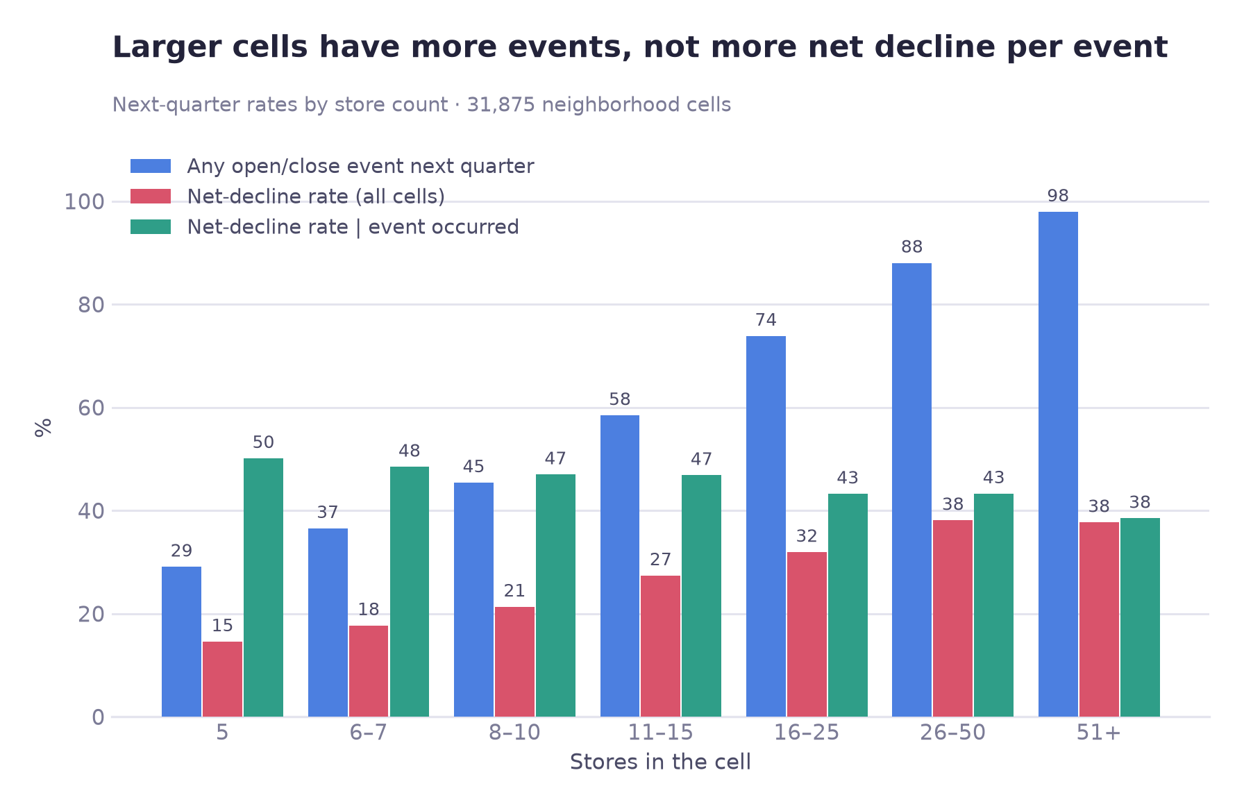
48.5% of these cells (15,451 of 31,875) recorded a zero because no opening or closure occurred (43.7% in the full 67,475-cell panel). A five-store cell has a 71% chance of no event in a quarter; a cell with 51 or more stores has a 98% chance of one.
Estimating store count's effect at each stage separately: it is concentrated in the first stage (coefficient +1.483) and small and not statistically significant in the second (+0.046, p = 0.114). After adjustment, store count is not shown to predict the direction of the balance once an event has occurred. The result therefore does not support “bigger cells are safer”; it indicates that the label mainly reflects how often an opening or closure occurs.
F · Differences in area-type sensitivity by category
Applying the test selected earlier (each category fixed, area types compared within it), the effect sizes range from 0.1202 down to 0.0002:
| Category | Effect size (ε²) | Reading |
|---|---|---|
| Pub / bar | 0.1202 | Highly location-dependent |
| Cafe / beverage | 0.0652 | Location-dependent |
| Korean | 0.0607 | Location-dependent |
| …six categories between | 0.048 – 0.016 | Weak to negligible |
| Chicken | 0.0002 | Area type explains almost nothing |
The two ends are ε² 0.1202 (pub/bar) and 0.0002 (chicken); the chicken value is statistically indistinguishable from zero (p = 0.355), so no ratio between them is quoted. Area type explains almost none of the variation in chicken shops' net-decline frequency (ε² = 0.0002), so area type is unlikely to be a useful basis for district-level targeting for this category; only the area-type classification was tested. One possible explanation is a high delivery share reducing location dependence, though nothing in this dataset measures delivery.
06
Results
Matched estimate, model performance, comparison with Seoul's change indicator and forecast
The matched ATT estimate
ATT
−5.57 pp
95% CI
−7.08 · −4.17
Pairs
7,043
Doubly robust
−6.00 pp
The interval comes from a commercial-area-level cluster bootstrap (853 commercial areas, 500 resamples); cells from the same commercial area recur across quarters and are not independent, and resampling them individually would understate the uncertainty. Across nine designs varying caliper width, replacement, exact-matching on quarter/district and seed, the estimate stays between −5.82 and −4.10 pp. A tenth setting that adds sales, which limits the sample to cells with observed sales (about 90%, 5,312 pairs), gives −3.65 pp; the sign is the same in all ten.
What −5.57 pp is an estimate of
An ATT, not an ATE: the average difference among the treated cells that actually exist (an adjusted association, not a proven causal effect), which matches the question of how the cells at the top of the ranking compare with similar cells. It is also restricted to the region of common support: 70.7% of treated cells were matched, and the unmatched 29.3%, which disproportionately include very large Korean cells, are excluded rather than extrapolated over.
Model performance
Aggregate ranking ability is only slightly better than store count alone (PR-AUC 0.418 against 0.388; AUC 0.669 against 0.654). The difference is larger when the model is used to select a short list, as shown below.
Top 50 · model precision
0.780
Top 50 · store-count rule
0.380
Smallest cells · model lift
1.548
Smallest cells · rule (mean over random tie order; range 0.73–1.34)
1.022
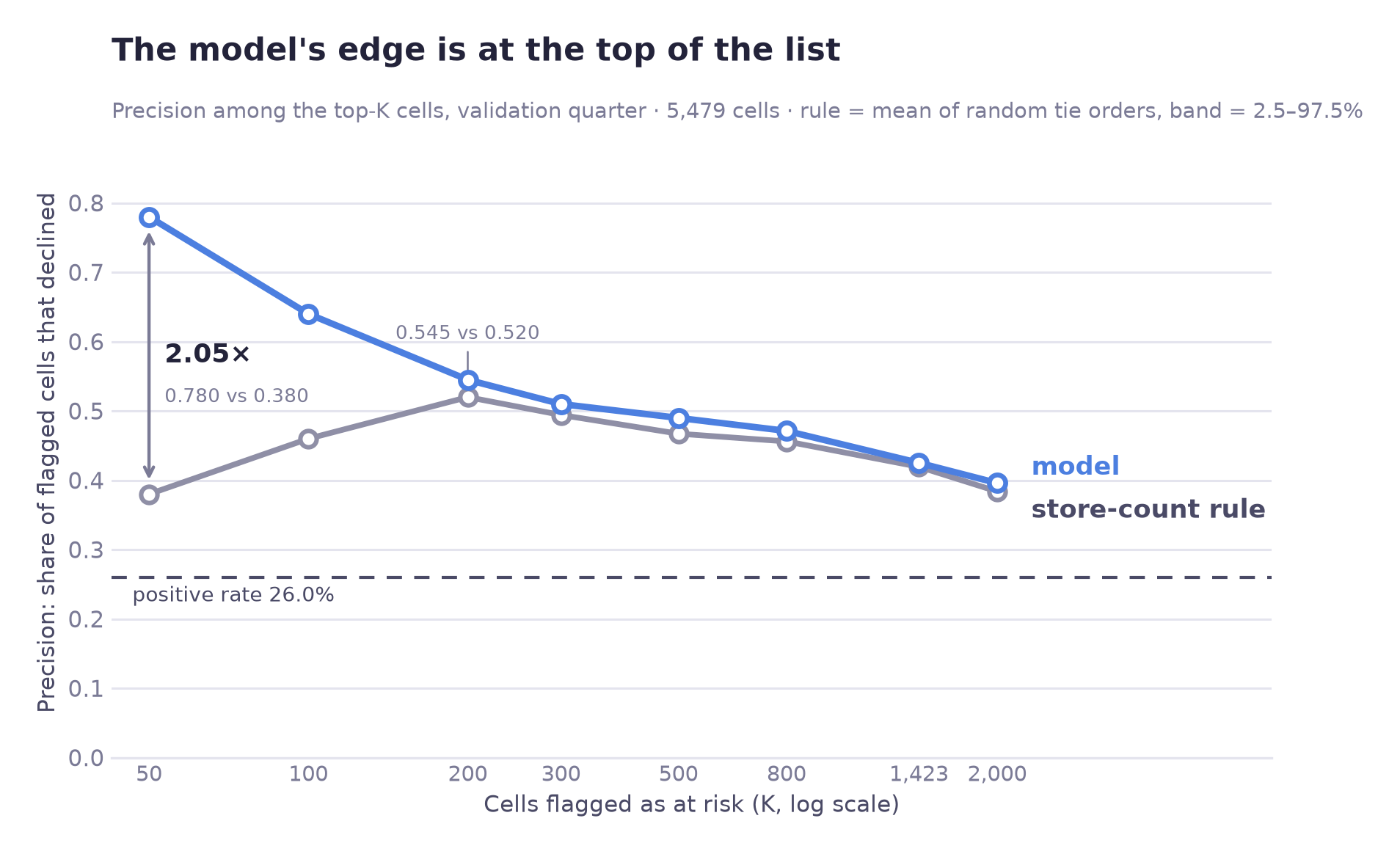
The 4% overlap at the top of the list indicates that the model is not simply reproducing the store-count ranking; if it were, the two lists would largely agree. Instead, 48 of the 50 cells it names are cells the store-count rule does not list.
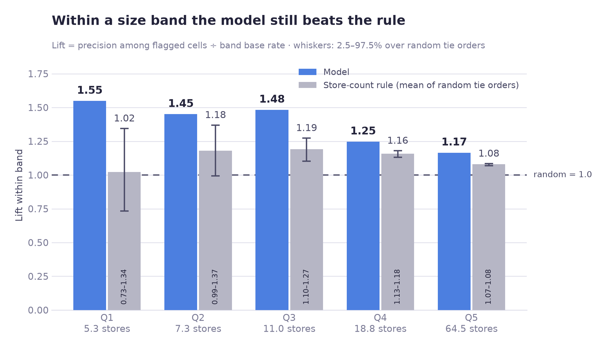
Summary of model performance
net-decline model: rolling AUC 0.666 ± 0.011 over 6 quarters · closure-count model (2,772 neighborhood cells, 2025 Q4 → 2026 Q1): top-decile lift 2.25× (store-count rule 2.18×), AUC 0.711 vs 0.705 for store count (+0.006)
The single-quarter validation figure is slightly higher, but the model was selected on that quarter, so it may be optimistic. The rolling number is the one reported, and the two agree to 0.003 (0.669 vs 0.666), though the rolling figure includes the validation quarter, so this is not an independent check.
Comparison with Seoul's published change indicator
Seoul grades each commercial district HH/HL/LH/LL by comparing the average operating months of its surviving businesses and of its closed businesses with the Seoul-wide averages in the same quarter. HL means survivors' average is above Seoul's and closed businesses' is below; the official description is that incumbent businesses in the area are competitive. The grade is published as reference information for business start-up and entry decisions, not as a net-decline forecast. This table tests one grade against this project's own label, which is not the indicator's published purpose. The source file has no category column, so each cell takes the grade of its commercial district (all ten food categories in a district share it).
Validation quarter: the 2025 Q4 grade joined to the 2026 Q1 outcome, 5,479 cells, all four area types. This is a single quarter.
| Seoul's change indicator | Cells | Net-decline rate | Lift |
|---|---|---|---|
| HL (label: “contracting”) | 974 | 24.3% | 0.937 |
| HH | 1,452 | 23.3% | 0.899 |
| LH | 790 | 22.9% | 0.882 |
| LL | 2,263 | 29.4% | 1.133 |
HL cells (the source file's label is “contracting”) had a slightly lower next-quarter net-decline rate than the average cell (24.3% against 26.0%; lift 0.937, close to 1), so HL gave no useful signal as a screen for net decline in this quarter. This is one validation quarter, so 0.937 should not be read as clearly different from 1. The indicator was not designed for next-quarter prediction; because it is built from closed businesses' operating months, using it as a feature could make the evaluation circular or leak target information, so it is used only as a baseline.
Category-level forecast
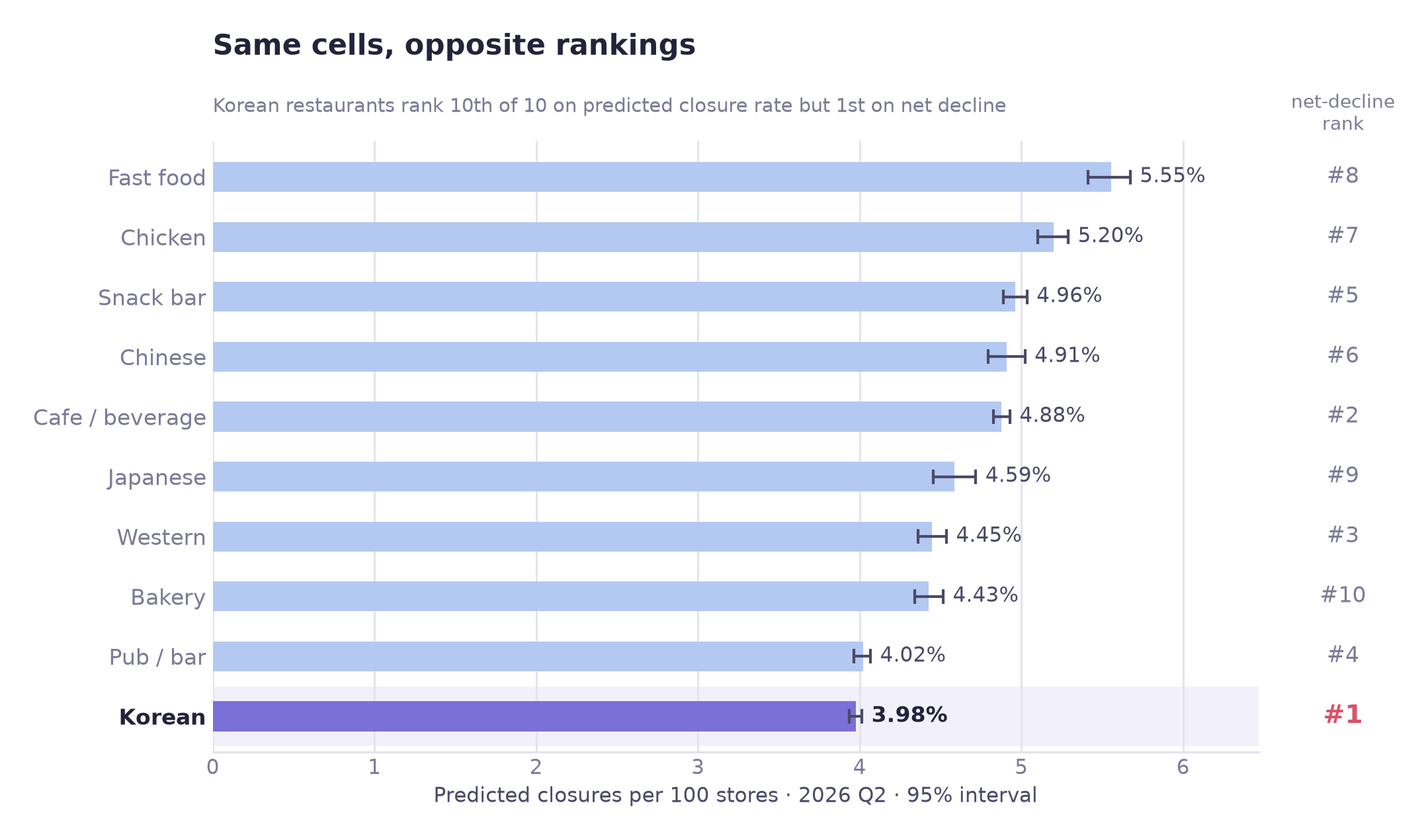
The forecast also illustrates how the two metrics differ. Rank correlation between the two predicted metrics (predicted closure rate and predicted net-decline probability, across the ten categories) is −0.370 (with only ten categories that is not distinguishable from zero, p ≈ 0.29). The category with the highest predicted net-decline probability finishes tenth of ten on predicted closure rate (point estimate; its interval, 3.94–4.01, overlaps pub/bar's 3.97–4.07). If support follows a net-decline ranking, the choice of metric could change who gets support.
07
Business insights
Implications of the results and proposed actions, under the assumed use case
① A net-decline ranking is closely tied to store count
The definition itself (closures outnumbering openings) can be met only in cells where events occur, which favours cells with many events. Korean restaurants' cells are large (21.3 stores per cell against 10.3 for the other nine), and holding store count fixed removes the modelled gap (+3.06 pp to −5.84 pp). The page does not split the top rank into a size part and a selection part: the 88% selection figure is measured against the all-ten average, the matched estimate against matched controls. In the single validation quarter tested, the HL grade of the city's change indicator was not a useful screen for next-quarter net decline either (lift 0.937, close to 1). Screening for net decline is not that indicator's published purpose, and the result should not be generalized to its other uses.
② Foot traffic and business turnover
Foot traffic is associated with both more openings and more closures. These data do not show a busy district to be a safe one; the pattern is consistent with fast turnover. And within a cell over time, changes in it are not significantly linked to openings or closures, so it may be standing in for fixed location traits rather than acting on its own.
③ The difference between Korean restaurants and matched cells depends on store count
Conditioned on measured circumstances, Korean restaurants have a lower net-decline rate than their matched controls in the three smallest size bands (−13.6 to −4.9 pp). In the two largest bands (Korean cells with about 16–24 stores, mean 19.6, and 24–142, mean 38.5) the interval includes zero. The difference depends on the combination of category and store count, which a category-level ranking cannot express.
④ Single-quarter city district × category rankings are not stable; the model was evaluated at the cell level
Ranked at city district × category from a single quarter (neighborhood cells, 2025 Q4 features, 2026 Q1 outcome), the rankings change when they are re-measured (split-half reliability 0.035 across 240 district × category cells). With six quarters pooled and only cells of at least 60 rows kept (97 cells) it is 0.259 (a different set of cells, so the two numbers are not a like-for-like gain). Cell-level scores are stored so the aggregation is possible, but a single-quarter ranking at that unit would be largely unreliable, so such a ranking is not reported.
⑤ The model's advantage is larger in smaller cells
On aggregate ranking it adds little over store count. Hold size constant and the store-count rule's lift falls to 1.02–1.19 while the model's stays at 1.17–1.55, with the widest margin in the smallest bands. The aggregate number alone would not show this difference.
Recommendations
01 Use cell risk scores rather than category rank, if support is allocated by risk
- Who
- Any district small-business office that allocates consulting or emergency loans by a category net-decline ranking (an assumed use case; no such rule is documented in this project)
- What
- If a category net-decline ranking is used, replace it with the top-K cell risk scores. Set K from the caseload an officer can actually contact, since precision falls as K grows.
- Evidence
- In the validation quarter, 39 of the model's top 50 cells had a net decline, against 19 for the store-count rule. The lists overlap by only 4%, so 48 of those 50 cells are not on the store-count list.
- Caveat
- This means the micro commercial district, not the city district. City district × category rankings were unstable in single-quarter data (split-half reliability 0.035 in one quarter; 0.259 for six pooled quarters among cells with at least 60 rows), so they are not shown.
- How to verify
- Two quarters later, compare supported cells against unsupported cells with similar risk scores as a comparison group
02 Show net decline together with closures per store
- Who
- Anyone building or quoting a net-decline ranking from open commercial-district data (net decline is this project's own label, not a published indicator; Seoul publishes openings, closures and the HH/HL/LH/LL change indicator)
- What
- Show closures per store beside the net-decline rate. The two rank the ten categories at −0.370 correlation (2026 Q2 forecast, from two different models; with ten categories not distinguishable from zero, p ≈ 0.29), so they do not agree on which categories are riskiest. In the single quarter tested, the HL grade (source label “contracting”) was also not a useful screen for next-quarter net decline, and it was not designed for that purpose.
- Illustration
- In the 2026 Q2 forecast Korean restaurants rank #1 on predicted net decline and #10 on predicted closure rate (model estimates, not observed outcomes)
- How to verify
- Ask dashboard users which categories are risky, before and after; or track how the figures get quoted in press coverage
03 Revise the foot-traffic advice in startup counselling
- Who
- District small-business centre counsellors; credit guarantee foundation consultants, where they advise prospective entrepreneurs on location
- What
- Where advice such as “choose a district with heavy foot traffic” is given, consider replacing it with “heavy foot traffic goes with more openings and more closures, which is consistent with fast turnover, so plan working capital accordingly.”
- Possible effect
- Possibly fewer under-capitalised openings in high-footfall districts (not tested here).
- How to verify
- 12-month survival rate of counselled openings, before and after the revision
04 Match the type of support to the category's location sensitivity
- Who
- Programme designers, if they are choosing between district-level and business-level support
- What
- Location-sensitive categories (pub/bar, cafe, Korean) are candidates for location diagnostics and district consulting. Categories with little location dependence (chicken, ε² 0.0002; fast food, ε² 0.0161, not significant after Bonferroni correction) are candidates for cost-structure measures instead, such as delivery commissions, franchise terms and operating efficiency.
- Expected effect
- Avoids assuming district-level support will move categories whose net-decline frequency barely varies by area type (not tested as an intervention). The gap in area-type sensitivity between the two ends is large (ε² 0.1202 for pub/bar against 0.0002 for chicken, which is statistically indistinguishable from zero, p = 0.355).
- How to verify
- Compare outcomes of district-level support for high- and low-sensitivity categories over four quarters
08
Limitations
What this cannot support
Aggregated quarterly counts cannot say which shop closed, and matching only balances what was measured.
Heterogeneity across size bands
The matched difference runs from −13.6 pp to +1.8 pp across size bands: clearly negative in the three smallest, with intervals that include zero in the two largest (Woolf p < .0001). The −5.57 pp average alone does not show that gradient, so the stratum table should be reported with it.
Scope
Matched estimates: neighborhood commercial districts, cells with five or more stores, ten food categories. The prediction models were fitted and validated on all four area types. Developed districts and traditional markets need refitting. The treated match rate was 70.7%, and very large Korean cells are disproportionately among those left outside.
Unobserved confounding
Matching balances measured covariates. Rent, owner age, tenure and capitalisation are absent, so the results are adjusted associations rather than proven causal effects.
The unit of observation
Data arrives pre-aggregated to district × category × quarter, so which shop closed cannot be determined. Much of the variation in closure counts probably reflects individual circumstances, which are not in the data.
Sales missingness is undiagnosed
The handling is conservative (excluded from matching, never imputed), but it was not checked whether the residual missingness correlates with the outcome, or what the 100% suppression rule actually is. The ATT does not use sales, so the exposure is confined to the prediction model.
An undocumented covariate
The area field has no definition in the source. The values suggest full polygon area rather than commercial floorspace; this is an inference, not a fact.
No sealed test quarter
The validation quarter was also used to choose the model. Six-quarter rolling validation stands in and the two figures agree to 0.003, but a genuinely sealed quarter would be better practice.
Reproducibility
Matching uses one shared seed (42) and stable tie-breaking. In a fresh-kernel check of the notebooks, two full runs produced identical CSV outputs (the two figures added afterwards were not part of that comparison).
What would move this forward
| Rank | What is needed | What it unlocks |
|---|---|---|
| 0 | No new data: re-match on within-category percentile | Tests whether the weakening of the difference in the largest bands is an artefact of matching on absolute store count. Cheapest open item, and the one most likely to change how −5.57 pp must be described |
| 1 | Business-registry event histories | Survival analysis instead of quarterly counts: “which shop, at what age” becomes answerable, and a risk window by tenure becomes actionable |
| 2 | District-level rent | Explains why store count matters at all. The available rent data is borough-level and has no discriminating power between commercial districts |
| 3 | Delivery-platform share | Tests whether the location-indifference of chicken and fast food is a delivery effect, which is currently only an inference |
| 4 | Staggered programme rollouts | Difference-in-differences, a design that can account for some unobserved confounding rather than only naming it |
09
Tools & Skills
What was used, and for what
Programming & data handling
Statistical testing
Matching and observational estimates
Modeling
Model evaluation
Visualization
Engineering practices
10
Repository
Notebooks, code, and full write-up
Code & outputs on GitHub →The repository contains twelve numbered Jupyter notebooks running end to end from the raw CSVs to the 2026 Q2 forecast and the figures (matching uses one shared seed (42) and stable tie-breaking; in a fresh-kernel check of the notebooks, two full runs produced identical CSV outputs, and the two figures added afterwards were not part of that comparison). It also contains the configuration module, the output tables and the full README write-up.